This article focuses on the importance of coaxial cables within high-speed digital signal applications, and how these cables relate to their far more abundantly recognized radio frequency (RF) applications. Coaxial cables can handle the increasingly higher frequencies used in digital protocols, such as USB4 and DisplayPort 2.0, along with 56 G and 112G PAM4 signals that are used in high-speed Ethernet within datacenters (1). To better understand the significance of coax cables, let us first examine their history and early applications.

History of Coax Cable

Coax cable has been around for more than 140 years. It was first patented in the United Kingdom in 1880 by Oliver Heaviside (see Figure 1). This “cable” was made with a rigid copper tube as the outer conductor and a copper wire as the inner conductor supported by discs made of an insulating material. The next improvement in coax design was patented in 1931 in the United States (2). This cable, created by Lloyd Espenschied and Herman Affel, was a flexible coaxial cable for use in the telephone industry. They focused on coax because its concentric design limits the effect of external noise on the transmitted signal, while also limiting the noise radiated out by its own signal.

In the years leading up to World War II, the United Kingdom used coax cables in their radio detection system; the term “RADAR” would come a few years later (3). In this time, Edward Bowen developed a more flexible coax cable using a new dielectric material the Imperial College of Chemistry created, polyethylene. His first segment of flexible coax cable was a short length of wire, coated in polyethylene of a set diameter, covered with braided copper and an insulation layer (2).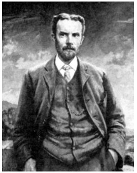   

RF Parameters 

What exactly are both these domains looking for in a coax cable, and how much overlap do they have? We will first look at the RF field and what some of their specified factors are. Some of these are quite common and straightforward, such as:

• Characteristic impedance
• Attenuation
• Rated frequency
• Maximum voltage and power
• Velocity of propagation

RF Parameters: Phase Stability

There are two additional quantities that have a broader impact on the cable, especially from the signal integrity field. These are the phase stability and voltage standing wave ratio (VSWR). Phase stability is related to the physical design of the cable as well as the physical orientation during operation; a geometric design (such as a coax cable) changes when it is bent, so one side of what used to be a proper cylinder is now a shorter path. While a characteristic is measured, it is very important to note the orientation of the cable and the physical design, or else every cable would behave the same. Everything from whether the center conductor is stranded or solid to how fast the jacket was extruded over the cable will affect this measurement. Other considerations include the dielectric material and how tight the shield is. The changes caused by bending are noticed as a phase shift at the output, hence why the measurement is called phase stability.

RF Parameters: VSWR

The VSWR is the ratio of the maximum and minimum voltage levels found on a transmission line. Ideally the ratio is 1:1, where the voltage on the line is simply what is transmitted. Each discontinuity in impedance along a transmission line causes a reflection of the signal, creating different maximum and minimum voltages.

The primary use of VSWR is in the RF domain. Particularly when designing the feedline for an antenna, the antenna itself has to be closely matched to minimize reflections. Reflected waves are power not being delivered to the antenna. They cause the line to reach a voltage above the transmitted level when they constructively interfere, potentially causing damage to the system (4).

VSWR vs. Return Loss 

How does the RF metric, VSWR, relate to signal integrity within the data communications world, and what other metrics might be used instead? For that I talked with Scott McMorrow from Samtec. VSWR is not used as much directly, instead return loss is used as a metric for cables and connectors and is typically measured in decibels. Return loss is a measure of the magnitude of the reflection, and it is one of several scattering parameters (5). VSWR and return loss are intrinsically linked and can be calculated from the following equation (6):

One small advantage VSWR has is that at low values it increases when connectors are added in series. In the design of cables and connectors, the VSWR is more difficult to control at high frequencies, so connectors rated for lower frequencies will often have a lower VSWR (5).

We will now take a look at parameters critical in the digital domain.

Digital Parameters: Scattering Parameters

The primary method for characterizing the signal integrity of a device is through its scattering parameters (S-parameters). These are a matrix of transmission and reflection coefficients between ports of the device.  Some of the most relevant ones are S₁₁, S₂₁, and S­₂₂. S­₁₁ is the reflection off the connector of port one, which is typically the input to the system. This value is also called the return loss and was defined earlier in the VSWR section. S₂₁ is the transmission coefficient from port one to port two; the inverse of this is called the insertion loss. S­₂₂ is the reflection coefficient off port two. These are just some of the main s-parameters used when looking into signal integrity. Though, the entire matrix fully defines the system (7).

Digital Parameters: Skew

The timing of a system is also critical to signal integrity. One measurement of timing errors is skew, which is related to the physical structure of the system. It is caused by differences in transmission line layout and composition between signals. When multiple signals are launched at the same time, such as a differential pair, the difference in their arrival time at the receiver is the skew. Another common occurrence of skew is in clocks; a clock signal needs to have synchronous arrival at all of the receivers to maintain the system timing.

Calibration and Verification 

It is important to note that the vector network analyzer (VNA) was calibrated very carefully (and verified) which is vitally important as the skew measurement is tied to the calibration reference plane of the VNA. Below in Figure 2 is an example calibrated VNA channel. Simple KF-KF connectors were used to connect port one to port two; the return loss was shown to be very low (-50dB) and the insertion loss was very close to 0 dB (typical specifications for a VNA is 0.1 dB max insertion loss variation out to 40 GHz).

Results in Practice

In practice what does it look like to gather these figures and prove signal integrity characteristics? I had the opportunity to learn about and witness part of the process during my internship with the company Wild River Technology using some of their cables, pictured above in Figure 3. At the time this post was written, these cable pairs were available for purchase as part of Wild River Technology’s ISI-USB4 Loss Modeling Kit (8). The process naturally started with SLOT calibration. One end of the cable was held in place while it was being measured. This VNA had two ports, so each cable in the pair had to be measured separately. However, the position that the end was held in remained constant. The cable was tested across a frequency range of 40 MHz to 40 GHZ. An example of the data from one of these tests can be seen below in Figure 4.

Figure 4 shows the s-parameters of one cable, as well as the calculated delay of each cable in the pair. With proper calibration and enough samples, this tool can calculate the delay down to the tenth of a picosecond, or 100 femtoseconds. (The method of calculating the delay to such a narrow degree and designing the cables around this calculation is currently proprietary.) This test setup could not measure both cables simultaneously, so skew could not be calculated directly.

The difference in the delay value between the cables is the relative skew between the pair. This pair of cables have delay values of 2.1336 ns and 2.1337 ns, respectively, so the relative skew is on the order of 100 femtoseconds. This is a very low relative skew and is achieved during manufacturing. One cable is created first and measured. The second cable is then cut as needed to match that delay, ensuring the relative skew between the cables is low.

The last component of testing I learned about was related to the lifespan of the cable. These cables are designed to be used for characterization testing in a lab, where they will be twisted and managed. Accordingly, the cable pair was bent a significant number of times, and the relative skew was recalculated at certain milestone counts of bends. This is a different bend method and more long term focused than the earlier phase stability testing. The data from when that test was run on the cable pair can be seen in Figure 5 and clearly demonstrates well behaved phase and insertion loss stability versus repeated bending.

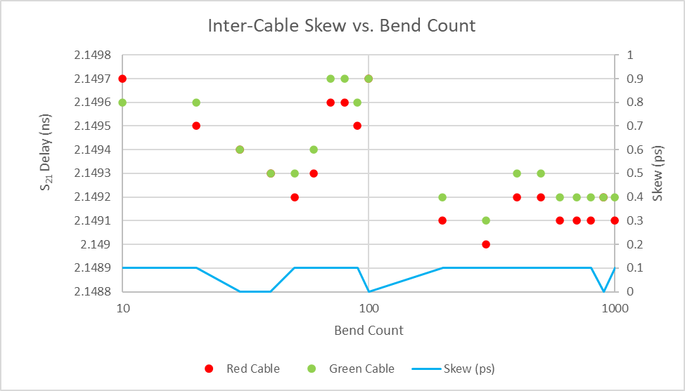Figure 5. Skew testing results for the cable pair

The cables are bound together by heat shrink to ensure they encounter the same physical stresses. This is critical to maintaining the tight skew matching of the pair in actual applications. Figure 6 shows how the cable pair responds to a substantial amount of simulated use. The cables are bent together during the test. Even after 1000 bends, the pair maintains a relative skew of 100 femtoseconds, well below the specified limit for USB4. The consistency implies that the cables will yield reproduceable measurements during testing.

Potential Applications 

The next part in this progression is the application, what will the cable be used for? Over the years digital communication protocols have been operating at increasingly higher frequencies, and the physical specifications for the test equipment have become even more rigorous. The equipment used to test these protocols must be able to measure the performance without interfering in the test itself.

High frequency testing is one possible application for coax cables, such as in the testing environment surrounding USB4. According to the USB4 Electrical Compliance Test Specification (Rev. 1.02) the cables used in testing must have phase matching of less than 5 degrees at 40 GHz. Phase matching down to this level is a narrow margin, translating to 347 femtoseconds. The cable pair measured in Figure 5 meets this specification (10).

In Figure 6, the light blue cables are all phase matched pairs. This setup is for calibrating the receiver for a stressed channel. The result will be used in error rate testing (9).

Conclusion

Digital and RF applications are both able to use coaxial cables as part of their implementation. They can even use the same cable, though the cables are typically described in terms of their RF use. Coax cables have a long and established history as a mainstay in radio applications and have been around for over a century. There are some similarities between the parameters for these systems, such as attenuation and insertion loss. There are also differences, such as the digital signal’s interest in eye diagrams and scattering parameters. This post looked at the digital applications of a coax cable, such as in testing USB4 implementations. There was also a focus on one pair of coax cables to highlight measuring some of their digital oriented parameters not always considered on an RF based datasheet.

Acknowledgements 

1. Al Neves – for being my mentor at Wild River Technology
2. Scott McMorrow – for very helpful conversation on VSWR and signal integrity engineering in general
3. Mike Engbretson – for very helpful conversations on testing and cable applications

References

1. Horner,Rita. “Shift From NRZ to PAM-4 Signaling for 400G Ethernet.” Synopsis, Synopsis Inc.
2. “History of Coaxial Cable.” Silver Comet Amateur Radio Society. 
3. “Coaxial Cable – 1929.” Magnet Academy, National MagLab, 10 Dec. 2014. 
4. Ulaby, Fawwaz T., and Ravaioli, Umberto. Fundamentals of Applied Electromagnetics. 7^th ed., Pearson, 2007.
5. Conversation with Scott McMorrow from Samtec
6. “VSWR / Return Loss Calculator.” All About Circuits. 
7. Bogatin, Eric. “How Not to Be Confused by S-Parameters.” Signal Integrity Journal, 7 Apr. 2020. 
8. Wild River Technology USB4 loss modeling kit
9. Images and testing information from Mike Engbretson of Teledyne-LeCroy