Often when simulating a serial communication link, we assume the majority of its components to be linear and time invariant (LTI).¹ Now, it is well known that LTI systems are completely characterized by their impulse response.² Furthermore, it is also well known that a system composed of two LTI components in series is also LTI, with impulse response given by the convolution of the impulse responses of its two constituent components:³

Therefore, if we know the impulse response of every component of our link then we may calculate its overall impulse response, using the above technique.⁴

Most link components have well understood impulse responses with convenient analytical mathematical descriptions. However, channel descriptions often come to us in the form of a series of samples of their frequency response, taken under certain well defined conditions.⁵ By far, the most common method of delivery of such samples is via the Touchstone® file format⁶

In general, Touchstone files may contain any number of ports. However, we will only consider two port models here. Touchstone files contain several pieces of information about a channel. The piece we’re interested in is the insertion loss, which also goes by the name: transfer function, often denoted as: . However, this equivalence between insertion loss and transfer function is only valid when the ports of the model are terminated into their specified impedances.⁷ The insertion loss of a two port Touchstone file is given in component S[2,1].

Note:  takes a real (and possibly negative) argument: ,  and returns a complex value:  
(), which gives both the magnitude and phase of the channel response at a particular frequency, .

Note: While H(f) is an analytical function valid for any value of f, the data we’re given in a Touchstone file is just a sampling of this function. Therefore, we may need to interpolate and/or resample the provided data, in order to make use of the function, H(f).

So, our problem statement is this:

Solution Description

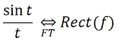
But, how do we do that? We know that the insertion loss is another name for transfer function, under the conditions stipulated above. And we know that the transfer function and impulse response form a Fourier transform pair:

So, maybe it’s as simple as: ?
That’d be great, since just about every mathematical modeling package out there has an ifft() function.

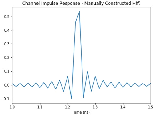
When we try this, we get a funny looking plot for the channel impulse response, which we know from experience to be wrong:

The problem is that the ifft() function expects its input to contain information about both the positive and negative frequencies within some magnitude range, in a very precise order:

where:

•   is the fundamental frequency,
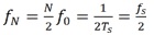•  is the Nyquist frequency,
• N is the number of vector samples,
•  T_s is the sample period, and
•  is the sample frequency.

The transfer function of any real structure, such as our channel, is Hermitian:

where  is the complex conjugate of 

And, so, Touchstone files do not bother toting around the negative frequency values, since they can easily be calculated from the positive frequency values, for any real channel. But we must remember to do this, before calling the ifft() function!

After properly massaging the original Touchstone data according to the above discussion, we get a more believable channel impulse response, which is shown in Figure 2.

That looks more reasonable, but where are those ripples coming from? Are they real?

Ringing

You may have already guessed that the ripples seen in the impulse response of Figure 2 are not real since, if they were, we’d have a non-causal channel and no real channel can be non-causal.

Let us look at the insertion loss data coming from our Touchstone file for this channel. Those data are plotted in Figure 3.

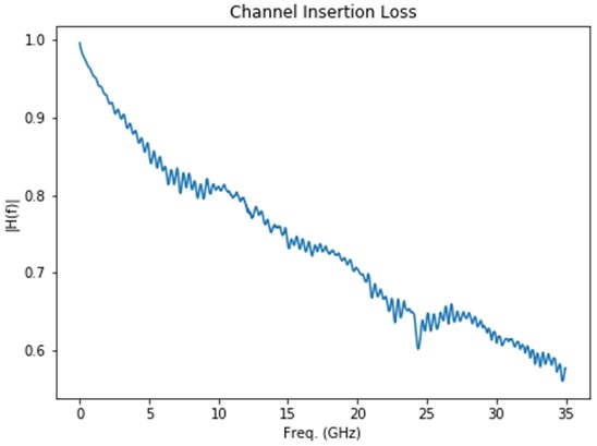
Notice that we simply stopped measuring the channel insertion loss while it still had significant magnitude! Clearly, the insertion loss didn’t suddenly drop to zero at the point where we arbitrarily decided to stop measuring it. But that is exactly what we are asking the ifft() function to believe. Indeed, as far as ifft() is concerned, the insertion loss of our channel looks like the plot shown in Figure 4. And one would expect that this might cause some problems in the results.

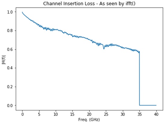
Note that the function plotted in Figure 4 can be expressed as:

where H(f) is our true channel transfer function and:

We find that our real channel transfer function has been windowed by a rectangular function, due simply to the finite frequency range of our measurement.

Multiplication in the frequency domain is equivalent to convolution in the time domain. So, we expect our calculated channel impulse response to be our actual channel impulse response convolved with the Fourier transform of the rectangular function, which is a sinc:

And this is exactly what we observe in the plot of Figure 2.

Windowing

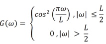
We can often reduce, if not eliminate entirely, the ringing observed in Figure 2 by applying our own additional windowing of the original frequency domain data, before transforming it into the time domain. The plot of Figure 5 shows one function commonly used for this purpose: the raised cosine.

The plot in Figure 6 shows the effect on the calculated impulse response (blue trace) of this additional windowing. In that figure, the calculated impulse response from Figure 2 is repeated (in gray), for reference.

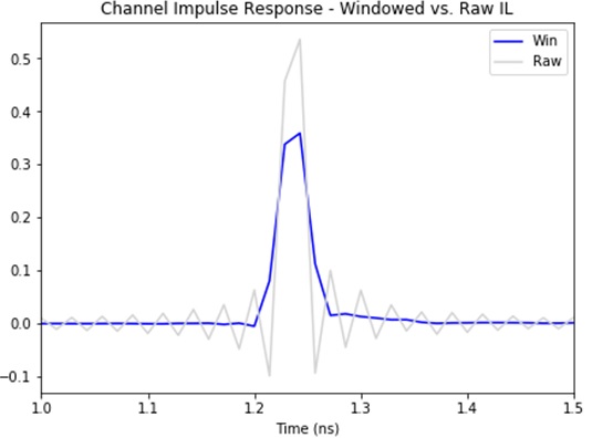
And we find that by preprocessing our insertion loss data with our windowing function we have eliminated the ripples, at the expense of reduced peak amplitude and slight broadening of the main pulse. (Nothing comes for free.)

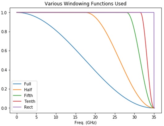
There are, of course, myriad choices for windowing functions. The plot of Figure 7 shows a partial family of raised cosine windows in which the active region is gradually narrowed from the full measurement bandwidth towards zero. The rectangular window implicit to the measurement data is also shown, for reference.

The plots in Figure 8 show the corresponding impulse responses.

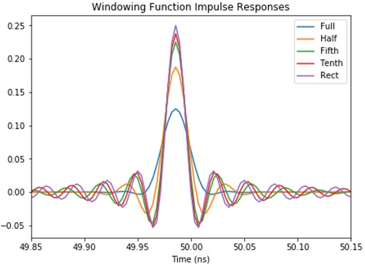
As is clear from both plots, as we reduce the width of the active region of the raised cosine window, its behavior in both domains asymptotically approaches that of the implicit rectangular window.

Closing Thoughts

We have looked at how we can convert channel insertion loss data in a standard Touchstone file into the channel impulse response, presumably for further use in time domain simulations. We have exposed the subtleties one must be aware of when feeding this raw measurement data into mathematical functions available in the standard modeling packages, such as ifft(). And we have shown how some pre-processing of the Touchstone data, in the form of windowing, can help improve our results, by eliminating the ringing that results from the use of frequency-limited measurement data.

The reader is encouraged to explore other windowing options for helping to optimize the conversion of insertion loss data into impulse responses. The author has found utility in the Hann window, for this application:

To this end, readers interested in further exploring this topic may find this Jupyter notebook extremely helpful: https://github.com/capn-freako/PyBERT/blob/master/misc/scikit-rf/S-param_Explorer.ipynb