
In power-aware parallel bus simulations, signal and power S-parameters are extracted together. Extracting signals without causality is well known in the literature. However, extracting power is causal, and extracting signal is also causal, so it is a challenging task because signal and power have different reference impedances.
A non-causal power delivery network (PDN) would possibly cause incorrect supply ripple voltage and incorrect signal swing during transient simulations. This causes the signal integrity (SI) engineer to incorrectly design a PDN, which has a cost impact to the product as well as design cycle impact.
This paper is a case study on causality problems in PDNs in power-aware SI simulations. Because power-aware IO buffer models (like IBIS 5.0) are used very commonly in simulations, extraction (S parameters) of package and board signals with power is becoming a challenge. Power integrity checks (DC drop or AC impedance analysis) will ensure that the PDN offers low impedance to IC drawing current to ensure ripple voltage is under control. This paper discusses the causality of PDN and the impact on design if a causality check is not done on the PDN for the package or board.
S-parameters with multiple reference impedances have become the default standard for SI-PI co-simulation modeling of PCB traces and planes as they accurately capture impairments such as crosstalk, reflections, and loss. For example, resonant behavior in systems is captured when working with S-parameters for signals, and impedance behavior is easily seen when working with Z parameters (converted from S parameters). While there are many advantages to using S-parameters for SI-PI co-analysis, there are certain problems associated with using them in time-domain simulations.
It is assumed that the Fourier transform is a precise means of converting from the frequency domain to the time domain. This would be true if the S-parameters were continuous and spanned all frequencies; unfortunately, this is not the real world case. Real-world S-parameters are bandwidth limited and sampled, so transformation into the time domain will result in non-causal signals.
Gibbs Phenomenon is one well known effect that causes a non-causal time domain signal and is due to the finite bandwidth of the S-parameter data set. Figure 1 below illustrates the same.

Causality
Causality is the property whereby a system only produces a response after it has received a
stimulus but not before. The goal of this work is to understand how causality violations arise in PDN networks during S parameter extraction when signals are extracted along with power and impact on PDN in power-aware transient simulations.
To understand causality violations, we need to separate them into numerical and non-physical components. Gibbs Phenomenon is an example of a numerical non-causality. Numerical non-causalities are caused by two separate attributes:
1. Real world S-parameters are bandwidth limited i.e. not infinity.
2. Real world S-parameters are a sampled data set i.e. it is not continuous; it is a discretized data set.
Non-physical components can be, for example, a full-wave simulation of a PCB trace that uses a non-physical dielectric model that can result in a causality violation.
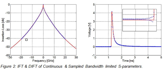
To simulate signals, simulation tools cannot work with infinite continuous signals; therefore, the infinite signals must be discretized. Time and frequency domain representations of the signals are linked through the Discrete Fourier Transform (DFT). Non-causality effects are introduced if this is not done with care.
Figure 2 compares the impulse response of an infinite continuous signal with the impulse response of a bandwidth limited discretized signal.
Extracting Causal S-Parameter Models
The frequency step/spacing of the S-parameter data can affect the causality of the data: the closer the frequency spacing, the better the S-parameter model. The maximum acceptable frequency spacing is determined by the delay and rise/fall time of the network being characterized.
The maximum frequency of the S-parameter data can affect the causality of the data. A higher maximum frequency will in general be better. It is sufficient to have data beyond the highest frequency that is relevant to the system bandwidth.
It is important to ensure that the frequency sweep begins at 0Hz, which is required by the nature of causality (tied to IFFT requirement), a true DC point.
The PDN for a package and board is usually modeled from DC to 1GHz (die capacitance dominates beyond 1GHz) with reference impedance of 0.1 Ohms. Signals are modeled based on their rise/fall times & data rates starting from DC with reference impedance being 50 Ohms. When both signal and power are extracted together, Fmax is dictated by signal Fmax for high-speed parallel bus interfaces.
It is bit tricky to follow the same rule for PDN (delay computation) with respect to frequency step as it is done for signals, as the PDN requires more samples up to 1GHz as compared to frequencies beyond 1 GHz. This ensures resonances (high impedance) are captured, and the PDN model is causal. This results in a non-uniform step size for low frequencies as compared to high frequencies. It is important to verify the causality of the PDN using industry standard simulation tools or Polar plots trajectory.
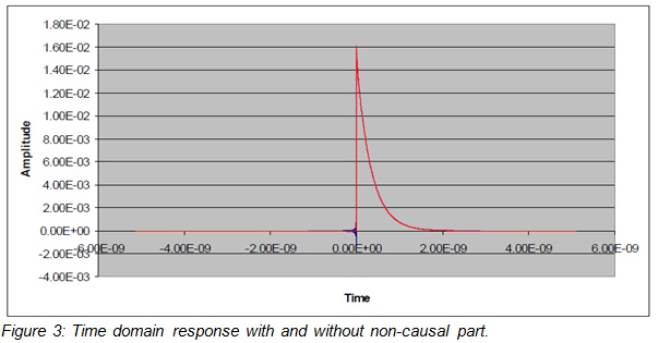
The time domain response can be made completely causal by setting all samples before time equals delay to zero. Figure 3 below shows the time domain response with and without the non-causal part. (Non-causal part energy is dependent almost entirely on the frequency spacing and insensitive to the maximum frequency.)
Cascading Causal Channel Models
In power-aware parallel bus simulations like DDR4 or Flash Interface, Controller package S parameters (Touchstone 2.0 version) are cascaded with Board S parameters along with Memory package S parameters as shown in Figure 4. Ensuring each of the S parameters is causal is not sufficient because the time domain response can still be non-causal.
It is recommended to cascade channel models with the exact same extraction settings with priority as follows:
- Same Maximum frequency Fmax
- Same Frequency step-size
- Integer Fmax i.e. No non-integer Fmax.
- Fmax should be an integer multiple of the step-size. This allows for ease of re-interpolation.
While cascading multiple channel models, the challenge of re-interpolating to a common step-size and then extrapolate to a common Fmax for purposes of IFFT in time-domain is one of the many challenges related to causality issues.

PDN Causality Effects on Time Domain Simulations
The previous sections showed how to extract causal models and the challenges in cascading multiple causal channel models. This section takes a closer look at the impact of non-causality of the PDN on supply ripple in the time domain.
The transient simulation setup as shown in Figure 4 is DDR4 1600MTps 8-bit wide PRBS7 with 50ps rise time data bus along with differential DQS (Data Strobe) flowing from controller (IBIS 5.0) to controller package (Touchstone 2.0) to board (Touchstone 2.0) to memory package (Touchstone 2.0) to memory (IBIS 5.0). Note that on-die de-caps for controller and memory are not considered as part of the simulation setup in order to capture the smallest effect of causality of the PDN.
In this setup, the controller package and board S-parameter extraction are user controlled while the memory package is used as-provided by the memory vendor (which is verified to be a causal model).
As a case study, two S parameter models are generated; one of them has PDN causal and the other has PDN non-causal. Note that the signal extraction is still causal, only the PDN is altered. Non-causality as a mathematical artifact is used (extraction setting) to generate non-causal and causal models. Non-causality is introduced on the IO supply rail of the PDN which connects the controller IO supply pins and the memory IO supply pins.
Figure 5 shows the comparison of ripple voltage on controller IO supply rail during a READ transaction for causal (red waveform) and non-causal (blue waveform) in the IO PDN case.
Note that the ripple waveforms are identical in terms of shape, but the amplitude is slightly lower for non-causal as compared to the causal case.

Figure 6 shows the comparison of the ripple voltage on the controller IO supply rail during a WRITE transaction for causal (red waveform) and non-causal (blue waveform) for the IO PDN case.
Note that the ripple waveforms are essentially identical in terms of shape, but the amplitude is slightly lower for non-causal as compared to the causal case.

Conclusion
This study dealt specifically with causality for PDN. It was shown how to generate causal models, issues with causal model cascading, and non-causal PDN effect on transient simulation. A non-causal PDN results in an incorrect supply ripple voltage. As a first order effect, an incorrect supply ripple voltage will result in an incorrect eye height on signal waveforms.
It is crucial to qualify PDN causality before moving on in the design. If a causality check is not performed, simulations may be flawed. Causality enforcement techniques can be applied to numerical non-causalities, but they will typically introduce unwanted errors in the S-parameters. Results of such enforcement may not be reliable, including the famous rational fitting process that most of the commercial tools perform either explicitly or implicitly.
This paper won an Outstanding Paper Award at EDI CON USA 2018.
Acknowledgement
Thanks to my manager Subhendu Roy for his valuable feedback.
References
[1] Stefaan Sercu, “Causality Demystified”, DesignCon 2015
[2] Madhavan Swminathan, “Causality Enforcement in Transient Co-Simulation of
Signal and Power Delivery Networks”, IEEE TRANSACTIONS ON ADVANCED PACKAGING, VOL. 30, NO. 2, MAY 2007
[3] Yuriy Shlepnev, “Quality metrics for S-parameter models”, DesignCon IBIS Summit 2010.
[4] Peter J. Pupalaikis, “The Relationship Between Discrete-Frequency S-parameters and
Continuous-Frequency Responses”, DesignCon 2012
[5] “Kramers-Kronig relation”, http://en.wikipedia.org/wiki/Kramers-Kronig_relations
[6] Philip A. Perry & Thomas J. Brazil, “Forcing Causality on S-Parameter
Data Using the Hilbert Transform”, IEEE MICROWAVE AND GUIDED WAVE LETTERS, VOL. 8, NO. 11, NOVEMBER 1998